FFT and LPC spectrum settings
Robert Mannell
a. FFT window length
In the following five images you will see the Fast Fourier Transform (FFT) and Linear Prediction Coefficient (LPC) analyses of the centre of the /i:/ vowel in the word "heed" spoken by a male or female speaker of general Australian English. The FFT is the grey jagged line and the LPC is the much smoother red line. In all cases the analysis of the male speaker is centred at time 0.557 seconds (relative to the start of the speech file). The difference between these male spectra is the length of the FFT analysis window (which, if you look carefully, also affects the LPC analysis). The analysis window is indicated by a pair of light blue vertical lines on the waveform in the bottom window of each image.
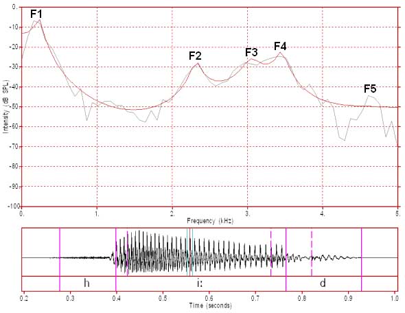
Figure 1: FFT/LPC of a male /i:/ FFT analysis window 12.8 ms (128 samples)
In figure 1 the analysis window is 12.8 ms (milliseconds). Since the sampling frequency (or sampling rate) is 10000 Hz for this speech sample, each sample is 0.1 ms apart. Therefore, 12.8 ms is equivalent to 128 samples (27 samples). Most Fast Fourier Transform analysis algorithms require an analysis window whose width in samples is a power of 2. This particular window is very narrow and is close to the period of one glottal cycle. As a consequence it does not capture the fine harmonic detail that can be seen when analysis windows exceed the duration of two glottal cycles (see below). Since this window length captures about one glottal cycle (not quite, because this is a Hanning window), it reasonably displays the overall shape of the spectrum. That is, the FFT analysis almost captures the shape of the spectrum in the region of the first four formants. In other words, the FFT spectrum is similar to the LPC spectrum around these peaks when the analysis window length is close to one glottal period.

Figure 2: FFT/LPC of a male /i:/ FFT analysis window 25.6 ms (256 samples)
In figure 2 the analysis window is 25.6 ms or 256 samples. In this case the analysis window is a bit more than two glottal cycles in length and so some of the harmonics can be discerned in the FFT pattern. However, because there are only 256 samples in the window and because the resulting FFT only consists of half that number of samples (ie. 128 samples) there is only 128 points of data available to display the spectrum between 0 and 5000 Hz. The separation between the data points on this spectrum is therefore 5000/128 or 39 Hz. Whether or not the harmonic spectrum is accurately displayed depends upon whether these 128 data points align with the harmonic peaks and dips. In this case they do so only partially and so we only get a partial indication of the harmonic structure of this spectrum. This window width is the MU-spec default for analysis of speech with a sampling rate of 10000 Hz.
This window width would provide a much better display of the harmonics of a higher pitched voice, such as that of an adult female, where the harmonics might be twice as far apart (and where there would be twice as many glottal cycles captured by the window).
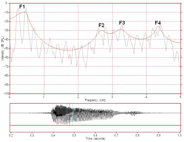
Figure 3: FFT/LPC of a female /i:/ FFT analysis window 25.6 ms (256 samples)
In figure 3 we have the FFT and LPC spectra of the vowel /i:/ spoken by a female speaker of Australian English. This FFT spectrum is generated from a 256 sample window and so there are 128 data points in the FFT spectrum. This is the same as for figure 2 but in this case the harmonics are 235 Hz apart (ie. the F0 is 235 Hz). This spacing is much greater than for the male voice, where the F0 is about 100 Hz (see text describing figure 4). With this harmonic spacing, 128 data points is more than enough to reliably display the harmonic structure of this speech sound. To calculate the F0 you should measure the frequency of a prominent harmonic. We will choose the 5th harmonic which has a frequency of about 1175 Hz. As this is the 5th harmonic, we then divide by 5 to obtain an F0 of 235 Hz. It is always more accurate to measure a higher harmonic and to then divide by the harmonic number. We could have chosen the 10th harmonic, which here has a frequency of about 2350 Hz and to then divide by 10 to obtain 235 Hz. It should be noted that 235 Hz is actually the average F0 of the six glottal cycles captured by this FFT analysis window. The F0 is actually declining over the course of the whole vowel from an initial value of about 250 Hz to about 190 Hz just before the stop occlusion and over the six glottal cycles in this spectrum the F0 declines by about 5 hz.
Note that the frequency range of 1 to 5000 Hz includes the first four formants for this female speaker whilst the same frequency range includes the first five formants for the male speaker (see figure 2). Also note that there appears to be a clear harmonic pattern all the way up to 5000 Hz.
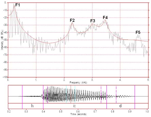
Figure 4: FFT/LPC of a male /i:/ FFT analysis window 51.2 ms (512 samples)
In figure 4 we have the same vowel as in figures 1 and 2 and the analysis window is centred at the same point, but the FFT analysis window is now 51.2 ms (512 samples) wide and captures about 5 glottal cycles. There are now enough data points to more accurately capture the harmonic spectrum which is an average spectrum for those five glottal cycles. We can also see that the 10th harmonic here is about 1000 Hz and so the F0 is about 100 Hz. As with figure 3, this is an average F0 across these five glottal cycles. If you look closely at the detailed harmonic structure of this spectrum, there seems to be evidence of harmonics up to about 3000 Hz. That is, there appear to be peaks at integer multiples of the F0 (100 Hz) up to about 3000 Hz although the pattern is really only clear up to about 2000-2500 Hz. Above this frequency the harmonic pattern appears to be increasingly obscured by noise.
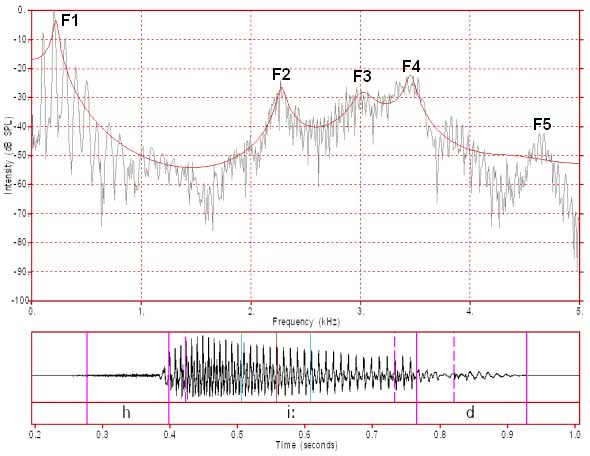
Figure 5: FFT/LPC of /i:/ FFT analysis window 102.4 ms (1024 samples)
In figure 5 we have the same vowel as in figures 1, 2 and 4 and the analysis window is still centered at the same place but now it is 102.4 ms (1024 samples) wide. It now seems that the harmonic pattern is only clear up to about 1300 Hz. It seems to disappear under noise above that frequency. Why is this so? Firstly, you should note that this analysis window captures about 10 glottal cycles and that over these cycles the F0 decreases from about 107 Hz to about 96 Hz. This spectrum is an average spectrum for those ten cycles and its harmonic pattern is averaged from those ten cycles. For the first harmonic, the range of actual harmonic values (ie. for each of the captured cycles) is 11 Hz (96 to 107 Hz). By the time we reach the 10th harmonic the range is 110 Hz (960 to 1070 Hz), by the 20th harmonic the range is 220 Hz (1920 to 2140 Hz) and so on up to 5000 Hz. If you closely examine the first 10 harmonics you will notice that they appear to get broader as we go from the first to the 10th harmonic. The harmonics then appear to break up as the range of frequencies for each harmonic becomes too great to permit the display of a single harmonic. This creates an increasingly spurious pattern as the harmonics for the individual cycles increasingly do not align. The greater the change in the sound during the analysis window, the more unreliable the spectrum produced. In this case the F0 has changed significantly during this window and so the harmonic spectrum is adversely affected. On the other hand, the formant pattern has remained steady so the formant pattern in this spectrum is still accurate. In the case of the female speaker in figure 3 the F0 only declined by about 5 Hz over the analysis window and so we have a clear harmonic pattern all the way up to 5000 Hz.
b. LPC Coefficients
As well as the analysis window length, the other main parameter affecting LPC spectra is the number of LPC "coefficients" used during the LPC analysis. In figures 1 to 5 we have used the MU-spec default value, which for a sample rate of 10000 Hz is 12 coefficients. 12 coefficients is theoretically supposed to give a good representation of 5 poles (poles are similar to formants). This values is determined by predicting the number of formants in the spectrum frequency range, multiplying by 2 and then adding 2 (the last 2 coefficients help to represent the spectral slope).
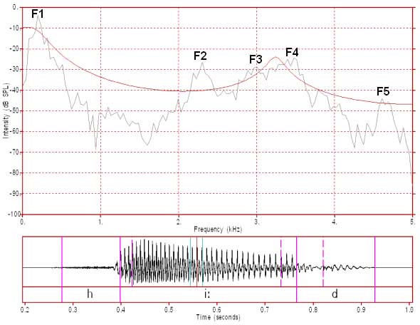
Figure 6: FFT/LPC of /i:/ with 4 LPC coefficients
In figure 6 we have only 4 LPC coefficients, which is normally supposed to only be adequate for representing approximately the spectral slope plus a single pole. In this case the single pole is centred over F3+F4.
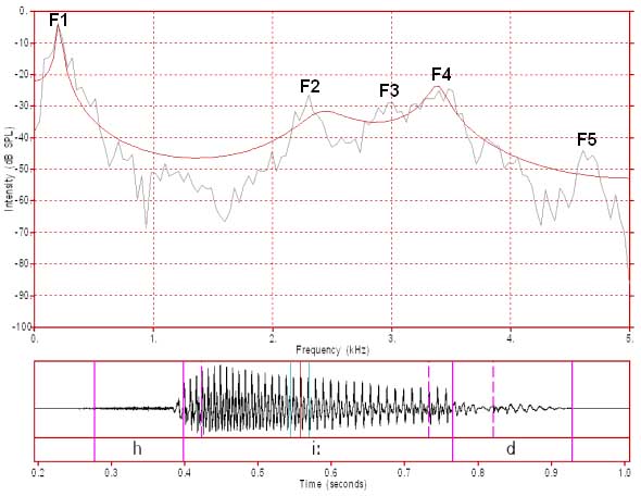
Figure 7: FFT/LPC of /i:/ with 8 LPC coefficients
In figure 7 we have 8 LPC coefficients. Eight coefficients should adequately represent the spectral slope plus three poles. In this case the poles coincide with F1, F2 and F3+F4. There are not enough coefficients to provide separate peaks for F3 and F4.
If you examine figure 2, above, we have the same window length as for figures 6, 7 and 8, but we have 12 LPC coefficients. This should capture the spectral slope plus all of F1 to F5, but for some reason F5 is not well modeled by 12 coefficients in this case.

Figure 8: FFT/LPC of /i:/ with 48 LPC coefficients
In figure 8 we have an LPC with 48 poles. This now provides us with a spectral envelope that closely hugs the top of the FFT harmonics, but it does not show the harmonics. If we increase the number of coefficients to 96 we start to see harmonics and with an even larger number of coefficients the FFT and LPC are almost equivalent. As we use LPCs in the algorithms that track formants (to produce the formant displays that we use in the vowel assignment) we need to define the correct number of coefficients that result in a peak for each formant but not in any additional peaks.
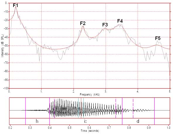
Figure 9: FFT/LPC of /i:/ with 16 LPC coefficients
A little bit of experimentation indicated that 16 coefficients is the smallest even number of coefficients that results in an LPC spectrum that captures all 5 formants and no other peaks for this particular analysis window. This 16 coefficient spectrum is displayed in figure 9.
c. Determining desirable linear prediction coefficient (LPC) filter order
(Please note: This section is not required reading for undergraduate speech and hearing students. This sub-topic is for more advanced readers.)
LPC analysis is a kind of signal filtering and the fineness of the analysis by an LPC is dependent upon its filter order (M). The "filter order" is another way of referring to the number of coefficients. That is, the "number of LPC coefficients" and the "LPC filter order" are synonymous.
Markel and Gray (1976, pp 154-156) recommend, for LPC speech analysis, choosing a number of coefficients (filter order "M") equal to the sampling rate in kHz, plus 4 or 5 additional coefficients.
Analysis bandwidth is always half the frequency of the sample rate, so if the sample rate is 10 kHz then the bandwidth of the resulting sampled speech is 0-5 kHz (0-5000 Hz). So, if we select 10 LPC coefficients for a signal with a 10 kHz sampling rate, this means that we have selected 10 LPC coefficients for a speech sound with a bandwidth of 0 to 5 kHz. Therefore, this means that there are two coefficients for each 1 kHz of the resulting frequency domain spectrum.
One pair of additional coefficients would be required to model the spectral slope (sometimes referred to as first spectral moment). Spectral slope is a consequence of both the shape of a single glottal pulse and the effects of lip radiation. Presumably the additional 2 or 3 coefficients recommended by Markel and Gray were considered desirable for modeling individual speaker variations in vocal quality, for dealing with the difficulty of analysing closely spaced formants (see below), and possibly the effect of antiresonances (spectral holes) on the spectrum.
For average adult male speech, resonances are spaced so that there is approximately 1 resonance per 1 kHz (at approximately odd multiples of 500 Hz). Since Markel and Gray were commenting upon analysis strategies that at the time were mostly applied to adult male voices, it can be seen that their recommendation was equivalent to a recommendation of 2 coefficients per resonance. For average adult female speech there is approximately 1 resonance per 1.2 kHz (at approximately odd multiples of 600 Hz). For children the spacing of resonances is even greater.
When we sample at low frequency rates, such as 10 kHz (10,000 samples per second) we will have a frequency band of 0-5 kHz. For an average adult male speaker uttering a neutral (mid-central) vowel there will be 5 resonances in this frequency range and this will result in 5 major peaks (ie. formant peaks) in the speech spectrum (at about 500, 1500, 2500, 3500 and 4500 Hz). As we need 2 coefficients for each of the five resonances plus 2 coefficients for the spectral slope then we will need a minimum of 12 coefficients to represent the 5 formants of the male speaker in this frequency range. The actual values of the first three formants of other vowels varies significantly from this but the average formant spacing is comparable to that of the neutral vowel. It should be noted, however, that for vowels with a pair of very closely spaced formants (eg. a close F1 and F2 or a close F2 and F3) an additional two coefficients might be needed to separate these closely spaced formants.
For an average adult female speaker uttering a neutral (mid-central) vowel there will be 4 resonances in this frequency range and this will result in 4 formant peaks in the speech spectrum (at about 600, 1800, 3000, and 4200 Hz). For this speaker we would need a minimum of 10 coefficients (4 times 2, plus 2 for spectral slope). Alternatively, we could change the sampling rate for the female speaker to 12 kHz (6000 Hz bandwidth) and in this case we would have 5 formant peaks in the spectrum at (about 600, 1800, 3000, 4200 and 5400 Hz). For this expanded frequency range we would need a minimum of 12 coefficients (5 times 2, plus 2 for spectral slope).
One of the advantages of adding an additional couple of coefficients, as recommended by Markel and Gray (ibid.), is that it doesn't greatly affect the analysis in a negative manner but does allow for some variation in speaker types and better handling of closely spaced formants for certain vowels. So, for example, 12 coefficients for LPC analysis of both male and female speech with a bandwidth of 5000 Hz works optimally for displaying the spectrum of the male speakers but isn't especially problematic for displaying the spectrum of the female speakers. This might only become an issue if we are trying to use the LPC analysis to track formants.
At higher frequencies, particularly above 5 or 6 kHz, the spectral correlates of the resonances tend to be attenuated (weaker or missing peaks) and so as sample rate increases above about 16-20 kHz the need for precisely 1 coefficient per kHz sample rate is reduced slightly. However, it should be noted that the choice of only 12 or 14 coefficients becomes increasingly error prone as the sample rate of the speech increases.
An example: 44.1 kiloHertz
If the sample rate is 44.1 kHz (standard CD audio) then the spectral bandwidth is 22.05 kHz (but rounded to 22 kHz for the remainder of this discussion). For adult male speech this results in 22 resonances between 0 and 22 kHz (although resonances are likely to be greatly attenuated in strength at higher frequencies and many will effectively be missing). Therefore 44 coefficients will be needed to account for these resonances. Adding 2 coefficients, to account for spectral slope, results in 46 coefficients. For adult female speech 18 resonances, and therefore 36 coefficients, are predicted based on the assumption of one resonance for each odd multiple of 600 Hz. This results in 38 coefficients for average female speech when the additional two coefficients for spectral slope are added. Rather than provide a different setting for an adult male and an adult female speaker a decision might be made to use the same setting, the 46 coefficient setting derived for the male in experiments comparing male and female speech. Smaller numbers of coefficients might also be acceptable, but this would need to be verified by experiment. For example, if we selected only 12 LPC coefficients for speech with a sample rate of 44.1 kHz then we would definitely fail to resolve the lower formants adequately. However, we might get good results for 36 or 38 coefficients but would need to test this experimentally.
Reference
J.D.Markel and A.H.Gray, 1976, Linear prediction of speech, Springer-Verlag, Berlin, 1976
Content owner: Department of Linguistics Last updated: 12 Mar 2024 10:42am