Analog and Digital Sound

Signals

It is very common for people who work in acoustics to refer to sounds as "signals" and to speech sounds as "speech signals". There is nothing mysterious about this terminology. The terms are interchangeable. The terminology arose amongst engineers who worked in the telecommunications industry in reference to the encoded sounds that passed over their networks.

Analog and Digital

In nature most phenomena have a number of properties that exist on an effectively infinite continuum of infinitesimally different gradations of change (exceptions to this can be found in quantum physics).

For example, we don't have 6 or so colours (eg. white, black, red, green, blue, yellow,...). We have a seemingly infinite gradation of colours. We don't have names for an infinite number of colours (although some people know an extraordinary number of colour names). We can certainly perceive a much larger number of gradations of colour than we can name. There is nevertheless only a finite (but very large) number of colours that we can discriminate between perceptually. There is an even larger number of colours that can be measured by spectroscopy.

Sound has properties (the dimensions of frequency, intensity, time and phase) that exist in the real world as infinite continua of infinitesimal changes. As with colour, this doesn't mean that we can name or perceptually discriminate an infinite number of gradations along these dimensions.

Phenomena that have such characteristics are sometimes referred to as "analog" phenomena. Sound can be said to be an "analog" phenomenon.

Strictly speaking, this isn't really correct. The word "analog" was originally used in this sense to refer to a transformed representation of a natural phenomenon. For example, sound can be represented by i) continuously changing radio waves, ii) continuously changing magnetic fields or electric voltages, iii) continuously varying physical distortions (eg. the bumps in the grooves of an old phonograph record). These representations consist of continuously varying properties are analogous to (or "analogs" of) the properties of the original phenomenon. In this sense, only these representations of sound are "analog" in that they are analogous to the original sound. Nevertheless, many naturally occuring physical phenomena, such as sound, are commonly referred to as analog.

"Representations" of sound are the result of transformations of sound into other analog or digital forms. Such representations are not sound, but sound can be recreated from these representations with the appropriate technology.

Until the invention of the digital computer all representations of speech sounds were analog signals.

Transduction

Transduction is the conversion of a signal from one analog form into another. Sound is transduced into an electrical signal by a microphone. In this electrical signal, continuously changing voltage is the analog representation of continuously changing sound pressure level. This electrical signal is transduced back into sound via a loud speaker.

A device that transforms a signal from one form into another is called a transducer. Microphones and audio speakers are transducers. The ear is also a transducer that converts sound into neural signals.

Digitisation: Sampling and Quantisation

When we sample an analog signal we measure the sound at (usually) equally spaced points in time. For example, if we want to digitise a sound so that it has the same quality as standard CD audio we need to measure the amplitude of the sound 44100 times per second. This gives us what is know as a "sampling rate" of 44100 Hz (44.1 kHz). We can't sample sound directly, but rather we sample the voltage of the electrical signal created when we transduce sound using a microphone. We can also choose to sample sound at other sampling rates. Higher sampling rates result in a more accurate match between the original analog signal and the resultant digital signal.

Sampling rate defines the temporal (time-based) accuracy of the resulting signal, but we also need specify the accuracy of the amplitude (sound pressure or voltage) dimension of the digitisation process.

The amplitude of an analog sound varies continuously between 0 and plus or minus some maximum amplitude (Amax). Amax is selected so that the signal is not "clipped". Clipping, or overloading, occurs when the maximum allowed quantisation value is less than the maximum value of the actual sound being processed. Once we have set the maximum value, we need to divide the amplitude range into a number of discrete amplitude steps between -Amax and +Amax. Sound data is stored in integers and integers on a computer (or an audio CD) are based on the number of binary "bits" in each sample. Early computer sound files were typically based on 8 bit numbers. This results in 2⁸ (or 256) discrete numbers that the amplitude scale can be divided into. As we have in a waveform both positive and negative numbers this means that all amplitudes in the original signal need to be mapped to the numbers -127 to +128. This is a very coarse mapping of sound amplitude and results in quality degradation readily audible to the human ear. Standard CD audio uses 16 bit numbers which results in 2¹⁶ (or 65536) values and the entire amplitude range of the original signal is therefore mapped to the numbers -32767 to +32768. If the maximum and minimum values are carefully selected then the resulting digital sound is almost indistinguishable from the original sound as the resulting quantised amplitude scale has a similar amplitude range to that of the human auditory system.

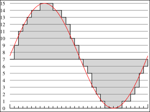
Figure 1: Pulse Code Modualtion (PCM). The horizontal (x) axis represents the points in time at which the analog waveform's smplitude is measured. The vertical (y) axis represents the amplitude quantisation values. The closest of these values to the red line is the selected quantised amplitude value. The resultant digital wave is a step shaped pattern which approaches the original shape as the number of quantisation levels increases.
Source: http://en.wikipedia.org/wiki/Image:Pcm.svg

Windowing

When we prepare digital speech signals for acoustic analysis we must first select a number of speech samples upon which we will carry out the analysis. As acoustic analyses attempt to extract the sine waves that add up to produce the variations evident in the waveform it is necessary to analyse more than one sample. One sample does not change and so there is nothing to analyse. Ideally, for a periodic waveform, at least two full cycles need to be analysed so that the spectrum display includes a frequency-domain representation of the periodic nature of the original waveform.

To select a series of speech samples for spectral analysis we need to "window" the original waveform. The simplest window is a "rectangular window". A rectangular window has a starting point "t1" and an end point "t2" with all values between t1 and t2 multiplied by one and all values before t1 or after t2 multiplied by zero. Figure 1 illustrates a rectangular window and its effect on a segment of speech. A rectangular window has a complex spectrum of its own which contaminates the spectrum of speech. A rectangular window is normally not used during the frequency analysis of speech.

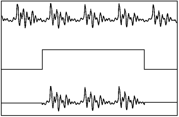
Figure 2: Rectangular window. The top panel shows the unwindowed speech. The centre panel shows the shape of the window (min. value = 0, max. value = 1). The bottom panel shows the resulting windowed speech.

A Hanning window is a member of a family of windows known as raised cosine windows. A single cycle of a cosine is inverted and shifted so that its values range between 0 and 1. A related window, the Hamming window, is slightly different to the Hanning window in that its values vary between 0.054 and 1 (so it is effectively a raised Hanning window). This class of windows has no significant effect on the shape of the spectrum of the resulting windowed speech and so these windows are often used during the frequency analysis of speech sounds.

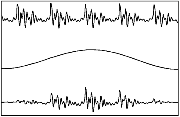
Figure 3: Hanning window. The top panel shows the unwindowed speech. The centre panel shows the shape of the window (min. value = 0, max. value = 1). The bottom panel shows the resulting windowed speech.

These are only two types of windows. There are numerous other types of windows.